
Much of the study of mathematics at more fundamental levels is dedicated to solving equations and systems of equations. In this article we will see how to use SymPy for these tasks quickly and intuitively.
If you prefer to watch in video, click on the player below. The complete article is found after the video.
Let’s start by importing SymPy and creating some symbols. We have already talked about creating symbols in the first article of this series on SymPy so, if you have any questions, take a look there.
import sympy


# settings for better outputs in the article, can be ignored
sympy.init_printing(
    use_latex="png",
    scale=1.0,
    order="grlex",
    forecolor="Black",
    backcolor="White",
)

x, y, a, b, c = sympy.symbols("x y a b c")
Using expressions and solve
Now let’s create an expression in the variable x:
expr = x**2 + 2*x - 8As we can see, the expression is of degree 2 in x:
expr
So, if we set the expression to zero, we will have a quadratic equation, the famous 2nd degree equation, and we could solve such equation. That is, find the values of x for which the equation has zero value, the roots of the equation. To do this, we use the solve method with the signature solve(expr, var), where var is the variable for which we want to solve the equation:
sympy.solve(expr, x)
Thus, we see that the roots of the equation x2+2x-8=0 are -4 and 2.
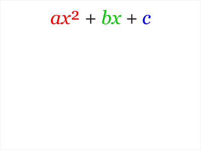
Now, the great power of SymPy is to be a symbolic CAS. Therefore, we can have the general expressions for the roots of a second degree equation written in the general form ax2+bx+c=0:
sympy.solve( a*x**2 + b*x + c, x)
Well, it is nothing more than the famous Bhaskara’s formula for solving second degree equations. The formula usually presented in books contains the symbol ± to indicate that there are two roots. Above we have the two roots in a more explicit form.
We saw earlier that the solution is presented in the form of a list with each root. Let’s then see each solution separately by accessing each item in the list in the usual way in Python:
solutions = sympy.solve( a*x**2 + b*x + c, x)solutions[0]
solutions[1]
Since lists are iterables, we can loop through replacing a, b, and c with the values used in the first expression of this article and verify that the roots are indeed -4 and 2:
roots = []
for solution in solutions:
    roots.append(solution.subs({'a': 1, 'b': 2, 'c': -8}))

roots
Using equalities and solve
The previous approach is perfectly correct and is widely used in scripts and tutorials that you find on the internet. However, there is another way to approach the problem that uses an abstraction of equality that exists in SymPy and that, particularly, I find more interesting because it is more semantic, closer to what we actually want to represent mathematically.
SymPy has the Equality class that aims to express the equality between two objects. There is the abbreviation Eq that makes it easier to write codes. Thus, the same previous expression, which we implicitly translated as an equation only when we did solve(expr, x), could be more explicitly recognized directly as an equation with:
equation = sympy.Eq(x**2 + 2*x - 8, 0)
equation
Note that now we effectively wrote it as an equation, with a left and a right side. The right side, in this case, being the number zero. Certainly this form is more easily understood.
And, of course, we can pass this equation to solve and obtain the same roots:
sympy.solve(equation, x)The right side does not necessarily need to be zero. The same equation could be represented by:
sympy.Eq(x**2 + 2*x, 8)
Which, obviously, would result in the same roots when passed to solve:
sympy.solve(sympy.Eq(x**2 + 2*x, 8), x)Systems of equations
We have already seen that we can solve an equation, but what about a system? We can easily. The first way is to pass an iterable of expressions to solve and also the variables of the system. Suppose a system formed by the equations x + y = 3 and 3x – 2y = 0. We could write:
sympy.solve((x + y - 3, 3*x - 2*y),
            (x, y))
Alternatively, we could be more explicit by creating each equation with Eq and passing to solve:
eq1 = sympy.Eq(x + y, 3)
eq2 = sympy.Eq(3*x - 2*y, 0)

sympy.solve((eq1, eq2),
            (x, y))
Be careful with floats!
Note that the result of the system came out in the form of a dictionary. And we can effectively substitute in any equation to see the result:
eq1.subs({x: 6/5, y: 9/5})
What does the result True mean? It means that the equality of the equation is satisfied. See the representation of eq1:
eq1
Thus, the True means that, when the passed values substitute x and y in the equation, the equality is satisfied, it is true.
Well, it would be expected that the same substitution in eq2 would return True, right?
eq2.subs({x: 6/5, y: 9/5})
Huh…?!
Be careful with floats! In the first article on SymPy we already addressed this a bit and saw how we can represent fractions in SymPy. See, when you write 6/5 in Python what you have is:
6/5
That is, a float. And operations with floats involve approximations, as we saw in the already mentioned article. Thus, it is worth transforming into representations of fractions of SymPy:
eq2.subs({x: sympy.S('6/5'), y: sympy.S('9/5')})Now we have the equality as valid.
Completing squares
Completing the square is a technique to convert a polynomial in the form ax2+bx+c to the form a(x-h)2+k for some values of h and k. It is used in several teaching contexts, the most well-known being in the derivation of Bhaskara’s quadratic formula.
In the animation below, we see that h=-b ⁄ (2a) and k= c-(b2 ⁄ 4a):
So we need to create two new symbols:
h, k = sympy.symbols('h k')We can, just as a didactic resource, express the equality by SymPy:
square = sympy.Eq(a * x**2 + b*x + c, a * (x - h)**2 + k)
square
Now, let’s take any quadratic equation and try to find the values of h and k. For example: x2-4x+7 = (x-h)2+k
square_example = sympy.Eq(x**2 - 4*x + 7, (x - h)**2 + k)
sympy.solve(square_example, (h, k))
Getting to know the Equality object better
Let’s take advantage and get to know the Equality object better with this example. So far, we have used it as a way to represent a mathematical equation, but we have already seen that the return can also be a boolean, True or False. Let’s understand.
First, let’s substitute the values found for h and for k in our object:
square_example.subs({h: 2, k: 3})
It is possible to obtain each side of the equality with the rhs (right hand side) and lhs (left hand side) attributes:
square_example.subs({h: 2, k: 3}).rhs
square_example.subs({h: 2, k: 3}).lhs
We can expand the square on the right side:
square_example.subs({h: 2, k: 3}).rhs.expand()Well, this shows that the two sides are effectively equal, right? Therefore, the following equality comparison should be true:
square_example.subs({h: 2, k: 3}).lhs == square_example.subs({h: 2, k: 3}).rhsFalse
Not! Why? According to the SymPy documentation, the library analyzes equality in form and not mathematical equivalence. For details, see this part of the SymPy documentation and this FAQ in the SymPy repository.
From what was seen, if the comparison is between the left side and the expansion of the right side, the result should be True:
square_example.subs({h: 2, k: 3}).lhs == square_example.subs({h: 2, k: 3}).rhs.expand()True
Right! And everything could be summarized in the following line, which instructs SymPy to make the possible expansions and check the equality:
square_example.subs({h: 2, k: 3}).expand()Conclusion and more articles about SymPy
The temptation to do any equation that appears in front of you with SymPy must be great now. Systems then, not to mention! But see how important it is to have a good mathematical foundation to understand what can be done with the library. Don’t skip math class (or even skip, but then study from the books ;-)).
If you want to know when new articles are available, follow Chemistry Programming on X. The complete list of articles about SymPy can be seen in the SymPy tag. And, if you would like to see all the tutorial series posts, see the SymPy tutorial tag.
See you next time.