Many consider mathematics, physics and the like to be difficult subjects, usually due to the traditional approach seen in schools. But the truth is that, shown in a more appropriate way, they are sensational areas and, if mastered, help us to give another view of the world. And computers can help in more complex and tedious steps of arithmetic manipulations. In this article, we will start to explore the SymPy library, taking the opportunity to make a good review of fundamental mathematical concepts.
Introduction and installation of SymPy
A computer algebra system (CAS) can be used for calculations with complicated mathematical expressions, solving equations, simulations, among other applications.
There are free systems such as SymPy and Octave, and commercial ones such as Maple, MATLAB and Mathematica. In essence, they all offer the same functionalities, so the choice falls on deciding technical and cost X benefit aspects, especially with regard to integrations with other tools. In this sense, SymPy has a great advantage, since the Python language is widely used in various contexts so that functionalities can be easily expanded. In fact, on the SymPy project site, these are the highlighted points:
- free, under the BSD license
- based on Python
- lightweight, with the only dependency being the
mpmathlibrary - is a library, can be used in other applications and easily extended
And the main reason for choosing SymPy, you can check your answers to the college calculus lists or those tests of teachers without creativity, with a lot of accounts and without any real application or contextualization 😉 Just don’t say I wrote that.

And if you are a teacher and the shoe fits, calm down and breathe. Obviously, the student needs to learn calculus, because if he doesn’t know the minimum, he won’t even know how to use the package, computers don’t work miracles, they return exactly what was requested. The criticism is about applying this knowledge in real cases. Create projects where the accounts are applied, create problem solvers and not human calculators.
SymPy is a symbolic computer algebra system. This means that numbers and operations are represented symbolically allowing to obtain exact results. Let’s understand this better.
Consider the number \sqrt{2}. In SymPy, such a number is represented by the object Pow(2, 1/2), while in numerical CAS, such as Octave, it is represented as an approximation 1.41421356237310 (a float). But so what? Well, depending on the application, there is no problem in having this approximation, but it can lead to problems. Let’s see an example.
If we use the sqrt method of the Python math package, we will also have the root stored as a float:
import math

math.sqrt(2)
1.4142135623730951
Now, we know that if we square \sqrt{2}, we should have the number 2, right? Let’s see:
math.sqrt(2)**22.0000000000000004
See what happened? There is a “4” lost there that, in a very simplified way, arises from the fact that the representation is an approximation.
And what is the consequence of this? We could list a few, but I’ll focus on one that catches many beginners by surprise. It is very common to use comparisons with == in conditionals or in function tests. These comparisons are at serious risk of failing when they involve floats:
math.sqrt(2)**2 == 2False
What to do in these cases? Well, if the context requires continuing to use numerical approximations and floats, a simple, but not always reliable way, is to compare with an acceptable tolerance in the context. For example, let’s say that an error of 1 in 10000 is acceptable in a given context. Thus, the test could be written as:
math.sqrt(2)**2 - 2 < 1E-4True
At some point I will write articles better addressing the care to be taken when working with floats, but at the moment there is this reading recommendation: arithmetic with floats from Python’s own documentation.
Let’s see how SymPy behaves in this simple example.
First, the installation can be done with a simple pip install sympy. If you use Anaconda, SymPy is already installed. The import is simple:
import sympyLet’s see what the representation of the square root of 2 looks like:
sympy.sqrt(2)
Note that the symbol \sqrt{2} appeared and not an approximation in the form of a float. Let’s do the squaring operation:
sympy.sqrt(2)**2
We obtained the exact result 2. We can even check that it is really the number 2 with the comparison:
sympy.sqrt(2)**2 == 2True
And, being the expression treated symbolically, it can be simplified symbolically. Remember that \sqrt{8} = 2\sqrt{2}? So:
sympy.sqrt(8)
SymPy took care of this simplification for you. And, more, symbolically this relationship is explicit, while if you do \sqrt{8} in your calculator or using a numerical package you will hardly realize that the result corresponds to 2\sqrt{2}:
math.sqrt(8)
We will now see the basics of mathematics with SymPy.
Basic mathematics with SymPy
Let’s understand how SymPy represents mathematical objects and simple operations. But first, let’s remember that in Python there are two main numeric types: integers and floats.
3 # int
3.0 # float
Floats are approximate representations of real numbers, up to the 16th decimal place. When we do a division, even of integers, the result is a float:
1/1
1/7
The integer division, represented by two bars, provides the integer part of the division:
1//7
While the % sign, known as modulo, provides the remainder of the division:
1 % 7
Rational numbers
Now, we know that 1/7 belongs to the set of rational numbers and its decimal representation is infinitely long. For an exact representation, we need the sympify method of SymPy:
sympy.sympify('1/7')
That can be called briefly S:
sympy.S('1/7')See how the fraction was passed to the method, as a string. Let’s see the type of the generated object:
type(sympy.S('1/7'))sympy.core.numbers.Rational
Therefore, the same fraction could be created as:
sympy.Rational(1, 7)Observe that in the form above the numerator and the denominator are passed as integers. We can do operations between rationals.
sympy.Rational(1, 2) + sympy.S('1/3')
A SymPy object divided by an integer results in a SymPy object:
sympy.S('1')/7Getting numerical approximations
During problem solving, it is better to obtain the numerical representation only at the end. To obtain the numerical approximation of a SymPy object as a float, we use the evalf() method. Let’s see an example with the number :
sympy.pi
type(sympy.pi)sympy.core.numbers.Pi
See that it is a specific type of SymPy, which has some numbers in its library. We will see some over time. Let’s see the representation as a float:
sympy.pi.evalf()
type(sympy.pi.evalf())sympy.core.numbers.Float
Observe above that SymPy has its own Float class (the same goes for integers and other types of numbers), not using the standard Python float. So be careful when mixing standard Python types and SymPy types. When in doubt, apply the sympify method already shown to ensure that everything is as SymPy objects.
A shortened way to call the evalf method is simply to use the n method:
sympy.pi.n()It is possible to request more decimal places. For example, if we want 50 decimal places for the number π:
sympy.pi.n(50)
This is possible because SymPy uses the mpmath library underneath, which allows calculations with arbitrary arithmetic precision.
There is also a global function N to obtain a numerical representation of SymPy objects:
sympy.N(sympy.pi)Since it is symbolic mathematics, we can use, for example, the notion of infinity, which has the curious symbol oo:
sympy.oo
sympy.oo > 100
Symbols
Since we are talking about symbolic algebra, nothing better than seeing how to create symbols with SymPy. From Python, we know that if we use some symbol not previously defined, a NameError will be raised:
x + 2--------------------------------------------------------------------------- NameError Traceback (most recent call last) Cell In[32], line 1 ----> 1 x + 2 NameError: name 'x' is not defined
From the moment we define x, it can be used. And, in Python, there is no need to declare the type of x:
x = 2
x + 2
The question is that we would like x to be recognized as a symbol. Think of the x from elementary school math classes, from the famous “find the x” or “solve the x” questions:

In other words, we want x with the classic meaning of a mathematical variable. We can do it as follows:
x = sympy.Symbol('x')
x + 2
Note that now it appears as a mathematical expression. We can create several symbols at the same time, notice that now the method is symbols:
y, z = sympy.symbols('y z')
x + y + z - 5
SymPy allows you to create symbols that follow a pattern. For example, in the study of polynomials it is very common to represent all coefficients with the letter a changing only the subscript number. This can be created with a representation very similar to the representation of slices of sequences in Python, in which the last number is excluded:
a1, a2, a3, a4 = sympy.symbols('a1:5')a4 * x**4 + a3 * x**3 + a2 * x**2 + a1 * x + 2
See that by default SymPy presents the polynomial from the lowest degree in x to the highest, leaving the term of for the end. It is possible to change the order by changing the monomial order instruction of the init_printing method, which sets how SymPy expressions will be presented. Let’s see:
sympy.init_printing(order='grlex')
a4 * x**4 + a3 * x**3 + a2 * x**2 + a1 * x + 2
grlex comes from graded lexicographic order, starting from the highest degree to the lowest, which is more usual in mathematical texts and the like. To return to the SymPy standard, we use the lex option:
sympy.init_printing(order='lex')
a4 * x**4 + a3 * x**3 + a2 * x**2 + a1 * x + 2
From the SymPy documentation, some letters are reserved and should be avoided as symbols: I, E, N, S, O, Q and C. N and S we have already seen. I and E represent the imaginary number i \equiv \sqrt{-1} and the base of the natural logarithm, respectively:
sympy.I
sympy.E
O is used for big O notation:
sympy.Osympy.series.order.Order
sympy.O(x**2) * x
C and Q have more specific uses, which are beyond the scope of this introductory material, but which can be seen in the documentation already cited.
Expressions
Expressions can be created by combining symbols with mathematical operations and other functions:
expr = 2 * x + 3 * x - sympy.sin(x) - 3 * x + 42expr
Note that the expression has already been presented simplified because it is a simple case of addition. In more elaborate cases, SymPy is not proactive in simplification, considering that it may be of interest to the user to obtain the raw expression, without manipulations. But it is possible to request simplification.
Simplifying expressions and obtaining coefficients
There is a specific method for simplification:
(x + x * y) / x
sympy.simplify(_)
The underscore _ takes the result of the previous cell and passes it to simplify.
Returning to our expr expression, it is possible to check the coefficients of the terms in x with the coeff method, assuming the expression as a polynomial in x:
expr.coeff(x)
Since the expression is of order 1 in x, there is no, for example, coefficient for a term of order 2 or, better saying, such coefficient is zero:
expr.coeff(x, 2)
If we want the 42 term in the expression, just request the coefficient of the x^0 term:
expr.coeff(x, 0)
It is also possible to check the coefficients relative to other terms, just treat them as if they were the variable of the polynomial:
expr.coeff(sympy.sin(x))
Factoring and expansion (distributive)
There are methods for various usual mathematical operations in expressions. For example, the factoring operation:
sympy.factor(x**2 - 2*x - 8)
And the opposite, the expansion or distributive multiplication:
sympy.expand( (x - 4) * (x + 2) )
It is also possible to make expansions of trigonometric expressions. For example:
sympy.cos(x + y)
sympy.expand(_, trig=True)
The collect method
When symbols are used as coefficients, SymPy does not join them. But we can use the collect method that collects terms additively with respect to a power. To understand, let’s create two symbols, a and b, and create an expression with them:
a, b = sympy.symbols('a b')expr = x**2 + x*b + a*x + a*bexpr
Let’s then pass the expression to the collect method, telling it to group the coefficients of the x^1 term:
sympy.collect( expr, x )
Observe that the expression was written in such a way as to make it explicit that the coefficient of the x term is (a + b). This can be useful in some contexts, especially for presentation.
However, even without writing explicitly, SymPy already recognizes the coefficient internally as (a + b), as can be seen with the coeff method.
expr.coeff(x, 1)
Substituting values in an expression
Something of great interest in the context of mathematical expressions is being able to substitute values to check the value of the expression after such substitution. Let’s create a new expression:
expr = sympy.sin(x) + sympy.cos(y)expr
With the subs method, we can pass a dictionary with the desired values for each symbol:
expr.subs({x: 1, y:2})
Note that the return was still symbolic, but we can see an approximation in float using the n method seen earlier:
expr.subs({x: 1, y:2}).n()
If the result of the substitution is exact, the return will be presented directly. For example, we know that \sin(\pi) = 0 and \cos(0) = 1. So the sum would be 1. Let’s see:
expr.subs({x: sympy.pi, y:0})
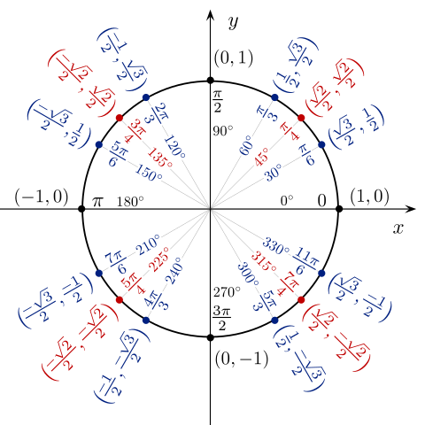
The same for other notable angles, which have symbolic representations. For example:
expr.subs({x: sympy.pi/2, y:sympy.pi/4})
If you didn’t understand, remember the notable angles with the following image of the unit circle:
In the case of requesting a substitution with already approximated values, we will have the following type of result:
expr.subs({x: sympy.pi/2.5, y:sympy.pi/4.3})
Conclusion and more articles about SymPy
In this article we saw the basics of SymPy and I hope it was possible to realize the power of this library. This is just the first of a series of articles about the library.
If you want to know when new articles are available, follow Chemistry Programming on social media. The complete list of articles about SymPy can be seen in the SymPy tag.